Getting Started: Incorporating Materials Management into a GHG Inventory
The first step in climate action planning is often to conduct a community-scale GHG Inventory. The main purpose of this page is to present some alternative inventory approaches - some simple, others more complex - for incorporating materials into these inventories. As background, this page begins with an introduction to inventories, summarizes how inventories traditionally treat materials and waste, and discusses some of the limitations of the traditional approach. The page ends with a few other considerations.
The focus of this toolkit is on community-scale inventories, not organizational inventories. Readers interested in organizational inventories (such as city government operations) are encouraged to review the: Climate Friendly Purchasing Toolkit 's page on conducting supply chain GHG inventories
Importance of Inventories: How They're Used
Inventories can be used for a variety of purposes. The primary purpose of a state or local community GHG inventory can be to:
- Help the community - including individuals and businesses in the community - understand its impact on climate change by demonstrating the community's main sources of climate pollution and/or how the community contributes to climate pollution;
- Daylight opportunities and responsibilities for emissions reductions through state or local policy and programs;
- Serve as basis for developing state or local community climate action plans; and
- Measure progress toward meeting state or local climate protection goals.
State and Local Inventory Protocols
At the state level, while there is no mandated protocol that states must follow, the EPA provides a "State Inventory Tool" (SIT) to facilitate development of state-level greenhouse gas inventories.
The dynamic is similar at the local level: there is no mandated protocol for local communities to use when measuring the carbon inventories or footprints of their communities, although the de facto standard in the US is the “U.S. Community Protocol for Accounting and Reporting of Greenhouse Gas Emissions” published by ICLEI.
Both the State Inventory Tool and CACP are geographic-based inventories, based loosely on guidelines developed for national GHG inventories. However, adjustments are commonly made to account for electricity (many communities purchase more electricity than they generate), and sometimes, waste disposal (for communities that are net importers or exporters of garbage). Even with these adjustments, these inventories are somewhat limited in their ability to accomplish the above purposes. As a result, some jurisdictions are exploring other methods for measuring their community's carbon footprint, such as consumption-based inventories, which provide alternative measures of the community's impact on climate change. What states and local jurisdictions are looking for in an inventory approach is a method (or methods) that is sensitive to changes in GHG emissions that the community can influence, emphasizes GHG emission sources that can be affected with state or local policy and action, clearly communicates and measures how the community contributes to GHG emissions and emission reductions, and has relevance to both policy and individuals.The State Inventory Tool is organized to produce a geographic-based inventory, focusing primarily on emissions sources located inside a state’s boundaries. This is largely consistent with guidelines developed for national GHG inventories. However, adjustments are commonly made to account for electricity (some states purchase more electricity than they generate), and sometimes, waste disposal (for communities that are net importers or exporters of garbage).
In contrast, the ICLEI protocol makes an important distinction between in-boundary emissions sources and activities resulting in GHG emissions, recognizing that many cities engage in activities that result in emissions that physically originate elsewhere. The ICLEI protocol provides a framework that encourages cities to first consider the goals and uses of their community-scale inventory, and then to choose which emissions to include (sources and/or activities) based on those goals and uses. The ICLEI protocol provides another innovation in that it recognizes that no single accounting or reporting framework can tell the full story of how a community contributes to emissions. It allows and encouraged the use of multiple reporting frameworks to tell stories suited to audiences and purposes. It also provides accounting methods for including emissions from materials and services used in the community, as well as an accounting framework for consumption-based emissions.
Going even further, ICLEI followed the publication of the community-scale inventory protocol with a supplemental “Recycling and Composting Emissions Protocol ” (“RC Protocol”). The RC Protocol is intended to help local governments account for the overall net emissions benefits of recycling and composting activities in their communities, as well as to estimate additional emissions reductions that occur outside the boundary of their community inventory.
Despite these recent improvements in protocols, many state and local inventories were first developed in earlier years, and greatly under-report the impact of materials. Even some newer inventories are continuing in this vein, perpetuating older inventory methods (“tradition”) and approaches. As a result, materials are provided only a very light (and incomplete) treatment, and many opportunities to reduce emissions are ignored.
Ultimately, what states and local jurisdictions are looking for in an inventory approach is a method (or methods) that is sensitive to changes in GHG emissions that the community can influence, emphasizes GHG emission sources that can be affected with state or local policy and action, clearly communicates and measures how the community contributes to GHG emissions and emission reductions, and has relevance to both policy and individuals.
Climate professionals often refer to inventories as tools that document the community's "sources of emissions". This implies a geographic view of emissions (sometimes called "the bubble") in which a community only documents the emissions that physically originate within their community ("under the bubble"). It is now common practice, however, to include emissions associated with combustion of electricity used in the community, even if these emissions physically originate in another community (wherever the generating capacity is located). A similar adjustment is sometimes made for waste disposal. It turns out that how we describe inventories is hugely important. If we say that "the inventory describes the community's sources of emissions", it implies the use of a narrow geographic approach, and excludes consideration of off-site emissions resulting from use of electricity and materials by the community (and in some cases, water and transportation fuels as well). In contrast, describing inventories as "characterizing how the community contributes to emissions" or “the community’s activities that contribute to emissions” opens the door to include consideration of these broader impacts, including materials management.
In response to the limitations of conventional inventories, some organizations have proposed the use of the phrase "footprint" to represent the community's broader climate impact. So while the inventory accounts for emissions that physically originate within the community, the footprint takes a broader view of all of the ways in which the community contributes to emissions (for example, through the use of materials). However, the terms "inventories" and "footprints" aren't well defined, and sometimes they're used interchangeably. If you hear the phrase "GHG inventory" or "community carbon footprint", the safest measure is to ask what they include, and what they exclude.
Background: How Conventional Inventories Treat Materials and Waste
Greenhouse gas (GHG) emissions occur throughout the lifecycle of the materials we consume. Energy is required at all stages, from raw materials acquisition and farming, to manufacturing and processing, to transportation and use, and finally to disposal. The lifecycle stages also have non-energy GHG emissions, such as process emissions from industry (e.g., perfluorinated compounds from aluminum production, CO2 from converting limestone to lime, CFC/HFCs from refrigeration) and methane from landfills. The graphic below illustrates these materials-related GHGs.
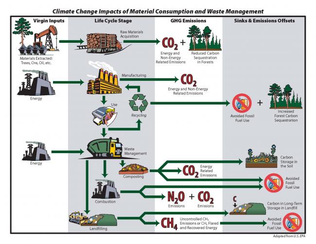
Of the materials-related GHG emissions in the graphic above, many inventories only take into account those from activities occurring within the geographical bounds of the community (and sometimes adjustments for electricity use and waste disposal). On the "upstream" end, these entail emissions from any raw materials acquisition, farming, manufacturing, or processing that take place within the community, as well as the associated transportation. On the "downstream" end, conventional inventories include landfill methane (CH4) emissions, incineration emissions (N2O and CO2 from any non-biogenic carbon such as plastics), and sometimes composting emissions. Conventional inventories do not account for potential sinks and emission offsets, although the EPA national inventory does keep track of them for informational purposes.
Limitations of the Conventional Approach
Of the materials-related GHG emissions in the graphic above, conventional inventories do not include "upstream" emissions from materials that are used in the community but not produced within its geographical bounds. Omitting these emissions from an inventory can limit the community from recognizing all of the ways in which it contributes to climate pollution. As a consequence, communities may miss opportunities and responsibilities for emissions reductions, in particular through materials management. This incomplete picture is perhaps the greatest limitation of the conventional inventory approach.
The conventional inventory can also lead to some surprising and potentially unhelpful results, if applied rigidly to climate action planning. For example, curbside recycling typically results in large emissions reductions when the collected recyclables displace virgin feedstocks in manufacturing. These emissions reductions may be many times higher than the emissions associated with collecting the recyclables (on-route emissions). For example, the Oregon DEQ has estimated that for Portland's curbside residential recycling program, the life cycle GHG benefits of recycling are about 40 times higher than the emissions associated with on-route fuel use. However, if a community only counts the emissions within their geographic area, they would count the on-route emissions but ignore the much larger life-cycle emissions reductions, and in the worst case, erroneously conclude that local recycling was a net source of emissions that should be discontinued.
Another example comes from efforts to encourage "low carbon purchasing". A bill introduced in the 2010 Oregon Legislature would have directed the state's Transportation Department to purchase "regionally produced" construction materials that contribute to a reduction in the state's greenhouse gas emissions. However, when it comes to materials, the state's inventory mostly counts the emissions associated with in-state manufacturing. Had the bill passed (it didn't), the consequence might have been that the state would buy materials produced somewhere else in the region, but not in Oregon because reducing production in-state would decrease the "state's emissions", while increasing production in-state would actually worsen (increase) the state's GHG inventory.
Again, however, the most important limitation of the conventional inventory approach is that it provides an incomplete view of how a community contributes to GHG emissions, and by extension, opportunities to reduce the associated climate impacts.
Conventionally, the GHG community has developed inventories using the lens of the traditional, sector-based view of in-boundary emissions. In this view, waste prevention and recycling are associated with the "waste sector", which typically appears as a minor or even trivial piece of the inventory. This is only reinforced by the common (although incorrect) perception that recycling and waste prevention are primarily about "keeping stuff out of landfills" and "extending the life of landfills". Yet most of the GHG reduction potential associated with prevention and recycling is upstream, in other sectors (manufacturing and resource extraction). For these reasons, it is much more useful to characterize waste reduction initiatives as "materials and waste" and to avoid the narrow and restrictive terminology of "waste emissions" or "waste initiatives". The "waste" element is important - and opportunities exist to reduce "waste" emissions both through waste diversion and better landfill controls. But "materials" are also important, and recognizing them helps to expand the conversation from the narrow frame of just "waste".
Alternative Inventory Methods
This section outlines several different approaches to account for materials in state and local community GHG inventories, beginning with easier methods and proceeding to more advanced or complex methods. It should be noted that many of these approaches supplement, rather than replace, traditional approaches. Put differently, they operate in parallel with a conventional inventory, rather than replacing it. This use of more than one reporting framework (in order to tell a more complete story of how a community contributes to emissions) is encouraged by the ICLEI Community Protocol and has been demonstrated by communities including King County (Washington), Portland (Oregon) and the State of Oregon.
Qualitative Method
The "qualitative method" involves adding a narrative discussion on the nature and significance of GHG emissions associated with materials to a GHG Inventory and/or Climate Action Plan. This qualitative presentation is used to give visibility to these emissions, which primarily fall outside the scope of the typical GHG inventory, and to provide the basis for adopting actions to reduce these emissions.
A good example of this approach can be found in an earlier Climate Action Plan for the City of Portland and Multnomah County (2009). A more recent update to Portland’s climate action plan adds a quantitative consumption-based approach, described below.) This qualitative approach and presentation can easily be adapted for use in any community GHG Inventory and Climate Action Plan.
A traditional sector based GHG inventory was conducted for the Portland area Climate Action Plan, which identified local energy use (residential, commercial and industrial) and transportation emissions as the primary sources of community GHG. The Plan is noteworthy, however, for also acknowledging the role of consumption of goods (and related emissions that are traditionally excluded from community GHG inventories). On pages 21 and 22, the Plan presents the EPA "sector" and "system" based views of emissions to make the following point:
- "Taken together, the traditional and complementary approaches to inventorying emissions offer insight into the underlying causes of - and therefore the opportunities to reduce - carbon emissions. Both approaches are needed because the businesses and industries located in Multnomah County produce different kinds and quantities of goods than what local residents consume. Examining carbon emissions through both methods therefore provides a more complete picture of the total emissions for which Portland and Multnomah County bear some responsibility."
Although Portland did not – in this version of its Climate Action Plan - calculate or estimate its own emissions resulting from consumption of goods, the inventory component of the Plan makes a compelling case for acknowledging and addressing these emissions. Materials management and consumption related actions were then incorporated into the Plan. Typical of more progressive Climate Action Plans, the Portland Plan includes a waste diversion goal - 90% diversion by 2030 - to increase recycling and composting. It also takes the innovative approach of including a goal to reduce solid waste generation - 25% reduction by 2030. This action is specifically intended to measure a reduction in material consumption by the community as a result of reduce/reuse strategies. In total, Portland's consumption and solid waste actions (includes those related to food consumption practices) account for 46% of targeted reductions to achieve the City's overall goal of 40% reductions in emissions by 2030.
Additional details on Portland's approach are provided here.
Another example of acknowledging the emissions associated with materials in a traditional inventory - without actually quantifying them - is provided in the State of Oregon's official inventory for 2004.
The qualitative approach has the advantage of being fairly simple and easy. It calls attention to the importance of materials and consumption without requiring any analytical effort. While probably not ideal, it is an easy and very powerful first step. Some additional suggestions for making this approach work:
- Early in the inventory discussion, note the emissions that aren't included (materials, consumption, other) and discuss their importance; don't relegate this to an appendix or a footnote.
- Provide quantitative examples from other communities, if possible.
- Qualify the traditional inventory as "Geographic-Based Emissions" or "Hybrid Production/Consumption Inventory", and don't characterize them as "comprehensive".
Per-Capita Method
The per capita method involves using national per capita GHG emissions derived from EPA's "systems" inventory and multiplying these emissions by the community's population. Like the qualitative method, the primary value of this method is to give visibility and relative significance to these emissions which primarily fall outside the scope of the typical GHG inventory, and to provide the basis for adopting actions to reduce these emissions.
EPA estimated that U.S. GHG emissions in 2006 were 7,054 MMTCO2E. This converts to per capita emissions of approximated 23 metric tons. This is substantially higher than the per capita emissions calculated from many community inventories since these inventories (at least for non-industrial communities) exclude emissions from industrial activities as well as some transportation emissions. EPA's systems inventory estimated that 42% of the nation’s emissions are associated with the provision of goods and food (collectively referred to as materials management). The per capita estimate for these emissions is 10 metric tons. To account for the lifecycle emissions associated with a community's materials consumption, the 10 tons per capita emissions for materials can be multiplied by a community's population to get a rough baseline of these emissions. This total can be compared with emissions from the sector inventory to give a more complete picture of the emissions that a community has some influence over (e.g., through their use of materials). Alternatively, a higher number could be used based on the UPSTREAM's adjustments for exports and imports.
In making this comparison it should be recognized that the industrial sector emissions estimated by the traditional inventory are a component of the materials consumption emissions derived from the national data. The main difference is that industrial sector emissions in a community are not correlated to materials used in a community and may be outside the influence local governments. It should also be noted that the inclusion of both local industrial emissions and national average pro-rated emissions for materials creates double-counting. As a result, it may be appropriate to adjust the per capita results and the discussion accompanying a per capita method needs to discuss this potential overlap.
From the perspective of materials management, the greatest advantage of this approach is that it offers a relatively simple method to use EPA's "systems-based" inventory of emissions and provide a quantified estimate for comparison with other estimates of emissions.
Depending on how emissions are pro-rated and adjusted, this approach might yield results that are less representative of local conditions than other inventory methods. In an extreme case, with all emissions pro-rated by a single variable (e.g. population) and no adjustments made, the resulting inventory would look exactly like the inventory for the US as a whole, only smaller.
One example of this approach is provided below.
Metro. The elected government of the Portland, Oregon metropolitan region has prepared a regional inventory - also called a "regional carbon footprint" - that is derived in part from EPA's systems view of GHG emissions. Metro's inventory shows results for three broad categories of emissions sources: transportation (of people), building energy use, and life cycle emissions for materials. It uses local transportation data to estimate the emissions associated with transportation of people. Emissions associated with building energy use are extrapolated region-wide from the Portland/Multnomah County GHG Inventory. Materials-related emissions are derived from EPA's systems-based view of emissions, with some adjustments made to reflect local conditions.
Material/Waste Flow Method
The Material/Waste flow method involves a more precise estimate of emissions associated with a set of targeted materials that are part of the material/waste stream in a community. It combines data from a waste characterization study or some other source to estimate that volume of specific materials used by a community with an emissions calculator to estimate the lifecycle emissions associated with each material. This method provides more precise estimates for the materials included, but it is not inclusive of many materials consumed by a community. This method has the advantage of creating a clear connection between the GHG inventory, the targets set, the actions taken, and the results measured when the proposed actions are associated with the materials included in the inventory.
Variations on this method follow this basic pattern:
1. The community estimates the quantity (in tons) of individual types of materials (corrugated, aluminum, food waste, etc.) used, generated, recovered (recycled, composted), and/or disposed of.
2. Use WARM or similar resources to identify emissions factors, expressed as emissions (or emissions reductions) per ton, by type of material/waste and management method. See the Setting Targets page for more information about WARM and similar resources.
3. Multiply the tons of materials/waste by the appropriate emissions factors to estimate emissions.
4. Sum emissions and, either add them to the conventional inventory, or hold them separate from the conventional inventory (depending on whether or not the same emissions are counted in both approaches).
This approach is included in the ICLEI Community Protocol as Appendix H, “Emissions Associated with the Community’s Use of Materials and Services – Accounting for Trans-boundary Community-Wide Supply Chains”.
There are several variations in how this approach can be used. Key variables include:
- Whether the community only estimates emissions for "readily recoverable" materials/wastes, or all materials/wastes
- Whether the community estimates emissions only for waste disposed, or for all waste generated (defined as disposal + recovery), or even more broadly, all materials used.
- Which life cycle emissions are included vs. excluded.
The following case studies illustrate different examples of the material/waste flow methods.
Ft. Collins, Colorado. The City of Ft. Collins changed its inventory method to include "upstream" emissions for the production of materials disposed of that are targeted for recovery in the City's Climate Action Plan. The City included these emissions without double-counting as none of the industrial or forestry activities are currently included in the City's conventional inventory.
State of Oregon (2004). The State of Oregon estimated some of the life-cycle emissions associated with a large variety of materials used in-state and included in waste generation, as part of an analysis for the Governor's Advisory Group on Global Warming. The analysis was used to compare the GHG emissions of various policy and program options against a "no change" scenario. The resulting emissions included significant overlap with emissions already included in Oregon's conventional inventory, and as such, the results were not integrated into Oregon's conventional inventory.
Denver. Researchers at the University of Colorado at Denver recently published a paper that estimates the GHG emissions associated with the provision of "key urban materials" for the City of Denver. These materials include water, fuel, concrete, and food. In the case of concrete, a materials flow method was used to estimate emissions.
Consumption Methods
A new and evolving approach to GHG inventories is to use a method that estimates lifecycle emissions associated with state or local consumption. These consumption inventory methods offer a radically different method of accounting for a community's contribution to greenhouse gas emissions. Traditional inventories evaluate the emissions associated with a diverse set of activities within a geographic area. These activities can include manufacturing, transportation of materials, transportation of people, use of electricity, use of energy for heating and cooling, and production of wastes. Some of the emissions - including emissions associated with electricity production and waste disposal - may occur outside of the geographic area. But typically, a traditional inventory focuses on emissions that physically originate inside the community.
A consumption inventory also involves a geographic area. Consumption activities within that geographic area are viewed as the root driver, or cause, of emissions. The consumption inventory includes only those emissions that are associated with consumption inside the geographic area. These emissions typically span the globe. Some will physically originate within the geographic area of the community, while many will originate elsewhere. Emissions physically originating inside the geographic area but not resulting from or associated with "consumption" inside the geographic area are not included.
It is important to understand what is meant by the term "consumption" and how this relates to materials use. "Consumption" is not the same as "use". Specifically, consumption refers to the purchase of goods and services by households and governments, and in some frameworks, also business purchases that are classified as investment or capital - typically, goods that are kept in inventory for more than one year, and not quickly passed on to another business. Other business-to-business expenditures - materials "used" by local businesses are not part of "consumption". For example, the purchase of a deep fryer (capital equipment) by a restaurant may be included as “consumption”, whereas the purchase of French fries are not. The reasons for this stem from the organization of national economic accounting systems, which inform the models that some consumption-based methods rely on. Regardless, the treatment of consumption means that when local businesses use such materials, the emissions associated with those materials are counted in a consumption-based inventory if the use is part of a supply chain that is satisfying local consumption. For a more detailed explanation of "consumption", click here.
Consumption inventories can be multi-regional, that is, trace supply chains through multiple regions, using different emissions factors for different areas. This allows for an understanding of which consumption-based emissions physically originate with the community, vs. other areas.
Consumption inventories are not the same as "systems inventories". For more explanation of the differences between these approaches, click here.
Consumption inventories are still relatively rare, although they are starting to become more common. Six examples are provided below of how this concept is being applied to GHG inventories.
DEFRA. The UK's Department of Environment, Food, and Rural Affairs commissioned a consumption-based emissions inventory for the years 1992 through 2004. It found that while the country's "conventional" GHG emissions fell by 5%, consumption-based emissions rose by 18%, partly a consequence of increased domestic consumption of imported goods with higher carbon footprints. This study also informed a provocative short video on “carbon omissions.”
State of Oregon (2011) . Oregon DEQ hired Stockholm Environment Institute to develop a consumption-based emissions inventory for Oregon for calendar year 2005. Results were published in late 2011. DEQ has subsequently updated the consumption-based inventory for calendar years 2010, 2012 and 2014 and Oregon now reports “in-boundary” and “consumption-based” emissions alongside each other as complementary inventory approaches.
King County and City of Seattle (2011). King County and the City of Seattle, along with the Puget Sound Clean Air Authority, hired Stockholm Environment Institute to develop both a "traditional" GHG inventory and a consumption-based inventory for Seattle and the larger King County. Results were published in 2012.
State of Washington (2006). Washington Department of Ecology hired Sound Resource Management Group to develop a Consumer Environmental Index (CEI). The model estimates emissions associated with household purchase, use, and disposal and provides a statewide index of climate change and ecosystems toxicity. While not organized or presented in the context of a greenhouse gas inventory, the methods used are fundamentally similar.
Denver. Researchers at the University of Colorado at Denver published a paper that estimates the GHG emissions associated with the provision of "key urban materials" for the City of Denver. These materials include water, fuel, concrete, and food. In the case of food, a consumption-based approach was used to estimate upstream (production-related) emissions.
Bay Area Air Quality Management District. Traditional consumption-based emissions inventories currently require extensive analysis, including the construction of a fairly complicated model. A household carbon calculator could be modified to estimate consumption-based emissions at the community scale. This is the approach researchers with the University of California’s CoolClimate Carbon Footprint Calculator used for the Bay Area Air Quality Management District, its nine counties and 110+ cities. Click here for more information on this approach.
Side note: treatment of recycling in consumption-based inventories.
In a consumption-based inventory, the emissions associated with producing goods are assigned to the community that purchases the goods (or causes the goods to be purchased, in the case of goods used in the supply chain). Emissions associated with disposal of goods by consumers (households and government) are assigned to the community the disposes of the goods. It is important to understand how this method of assigning emissions treats emissions reductions resulting from community-scale recycling programs. Click here for details.
Other Inventory Considerations
Waste disposed by the community, not in the community
Many communities send their wastes for disposal in a landfill or incinerator located in a different community. Some communities may be hosts to such facilities, which are accepting wastes from multiple jurisdictions. An important question is: how to account for these emissions?
In the case of a community that sends its waste exclusively to facilities that are not owned or located in the community, the most straightforward approach is to estimate the emissions associated with only the wastes disposed of that originated in the community.
If however the community (state or local government) is home to a disposal site that is owned, regulated, or otherwise overseen by the community, then it might make sense to account both for the emissions resulting from disposal of waste generated by the community (regardless of where the disposal occurs) as well as all (other) emissions from the facility located within the community. For example, Oregon is a net importer of waste from Washington state. Oregon estimates two separate numbers for waste disposal: emissions from disposal of all waste generated inside Oregon, and additional emissions resulting from in-state disposal of waste originating in other communities. The former number is influenced by both waste reduction and landfill controls; for the latter number (waste imports), Oregon's influence is limited primarily to landfill controls.
ICLEI’s Community Protocol requires that communities, at a minimum, estimate the emissions resulting from the generation of solid waste by the community, regardless of whether the waste is ultimately disposed of in the same community or somewhere else.
Gas capture rates
There are at least two outstanding issues with regards to how models for estimating landfill methane emissions treat gas capture.
- Little agreement exists on values to be used in the absence of site-specific numbers. According to the EPA, the average US methane recovery for both MSW and industrial landfills, representing landfills with and without gas capture systems, was 44.8% for 2005. For facilities with recovery systems in place, EPA’s AP-42 (1998) recommended 75%, based on estimated collection efficiencies between 60 and 85%. More recent analysis conducted in support of EPA’s WARM tool (2016) suggests average US collection efficiencies of 64.8%, with a range from 60.3% (“worst case collection” under EPA New Source Performance Standards) to 78.8% (the “California regulatory scenario”). IPCC (2006), recommended a 20% default as an international default to incorporate landfill gas collection rates from those countries which currently do not have regulatory systems in place. Actual values are sensitive to cover type, percentage of landfill covered by the recovery systems, presence of liner, open/closed status, type of waste, precipitation, and other factors.
- Simple models assume that gas capture is a constant percentage of generated methane, over time. The application of a one-time average recovery rate introduces errors that likely understate actual methane emissions. Once anaerobic conditions are established, organic matter tends to spike in methane emissions. The period prior to the activation of any methane recovery system therefore can result in high methane release, particularly for organics, that would not be accounted for in most simple models. Models assuming constant gas capture rates also fail to account for emissions after the landfill is closed. This explains some of the differences between EPA’s higher (1998) and lower (2016) estimates; EPA’s more recent analysis includes estimates of methane emissions that occur prior to the installation of gas collection systems, as well as emissions after the gas collection system is turned off.
Click here for additional details regarding gas capture rates.
Treatment of energy recovery from waste (avoid double-counting)
Waste incineration for energy production can replace fossil fuel use. Whether waste incineration leads to lower emissions than fossil energy depends on (1) the waste's energy content, and (2) whether it is biogenic (biomass, such as paper and wood) or non-biogenic (fossil-derived, such as plastic). Since biomass carbon would eventually decay and emit CO2, CO2 from burning biogenic waste is not included in most conventional inventories. Thus, energy recovery from burning waste with high energy content and/or biogenic content can sometimes lead to lower emissions in an inventory, compared to fossil fuel energy use.
The potential exists for double-counting for emissions from both landfill (landfill gas) and incinerator waste-to-energy. If the waste-to-energy facility is producing electricity or fuels that are subsequently used in the community, those emissions may be counted in the "electricity", "built environment", or "transportation fuels" portion of the inventory. Also counting them as "waste" emissions would result in double-counting. Communities should count these emissions only once. In the case of electricity generation from waste, communities need to decide if they want to count all emissions from the waste-to-energy activity, or treat the emissions as part of the resource mix for their regional electrical grid.
Use of 20-Year Global Warming Potentials
Methane has a shorter lifetime in the atmosphere than carbon dioxide. Its warming effect is therefore concentrated in the years immediately following its release, more so than carbon dioxide. Global warming potentials (GWP), which express the contributions of gases (relative to carbon dioxide, which is defined to have a GWP of 1) reflect this.
- The 20-year GWPfor methane is 84 (without climate-carbon feedbacks).* On a 20-year horizon, the same mass of methane, compared to carbon dioxide, is 84 times more potent in its greenhouse effect.
- The 100-year GWP for methane is 28.* On a 100-year horizon, the same mass of methane, compared to carbon dioxide, is 28 times more potent in its greenhouse effect.
*Note that these values are based on the IPCC's Fifth Assessment Report (2013), the most recent "official" estimate of global warming potentials by the International Panel on Climate Change. However, EPA and many other organizations continue to use global warming potentials from the IPCC's Second Assessment Report (1995), where methane was estimate to have a 100-year GWP of 21. As our understanding of climate science improves, the global warming potentials are periodically updated, and IPCC may yet again revise GWPs in future assessment reports.
Traditional inventories typuically use 100-year GWP values, since carbon dioxide's atmospheric lifetime is on the order of 100 years. Yet 20-year GWP values allow for an alternate view that highlights reductions that will have a greater climate impact in the short-term, and can provide valuable insight for policy makers. The best approach may be to conduct inventories using both sets of global warming potentials so that policymakers can understand how the community is contributing to global warming in both the short run (which is important) and also over a longer time period (which is also important).
Consideration of Timing
Some materials management practices can result in emissions - or emissions reductions - in future years. Landfilling, and avoided landfilling, are two examples. Composting food waste in the year 2010 will reduce landfill emissions in 2010 and for many future years. The forest carbon sequestration benefit from source reducing and recycling paper is another example of a benefit that reduces emissions gradually (as trees grow) for years into the future. This is significant, since inventories typically portray emissions in the year in which they occur. EPA's WARM tool reports emissions factors in aggregate, rolling current and future emissions (and emissions reductions) into a single number. Communities may need to disaggregate these emissions (and emissions reductions) into the years in which they actually occur. For more information on this approach, click here.